Improved Chlorine Residual Control

by Cliff Laver, P.Eng

Investigation

In this post, we’ll describe replacing an old stand-alone Cl₂ controller that was being used by a municipal water system. The old system was cumbersome and difficult for the operators to use; performance was poor.

A review of the site in question showed that there was a SLC PLC controller already present. There were spare analog I/O on the controller and the flow rate as well as the residual were being fed back to the PLC.

Overview of the Stand-Alone Controller

The stand-alone controller did not have much information available as to its exact functionality. It was old and falling apart. The display on one of these controllers was non-functional. There were some convoluted manuals on how to use the PID features. The controller was not maintaining a constant Cl₂ residual, it would fluctuate and have difficulty maintaining the setpoint. Support was non-existent.

Objective

The municipality wanted to have a reliable control of the Cl₂ residual. They wanted the setpoint to be maintained at a constant rate in order to reduce Cl₂ costs and reduce health concerns. They also wanted to grant the operators the ability to change the residual with ease.

Testing

As there was a SLC505 PLC onsite, it seemed like this would be fairly straight forward; replace the functionality of the stand-alone via the SLC. The first step was to learn about the system; this was accomplished with an open-loop bump test.

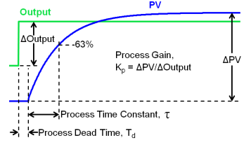
Figure 1 – Open loop test (Coughran, 2018)

Where CO is the Control Output

Where PV is the Process variable

Where Td is the dead time

Where Tau is the process time constant

Where Kp is the Process Gain

To perform the test, make sure that the system is relatively stable (no surging flows, etc..), then place the system in manual and increase the control output (CO) by about 10%. Figure 1 shows all the variables that are needed and where they are located.

The point is to give a starting point for the SLC PID to take over control. The following results are displayed below:

Td = 93s, Tau = 32s, ?PV = 38.4%, ?CV = 15% and a calculated Kp of 2.6

I know from my control theory classes that when Tau > 2Td most tuning will work well but when Td > 2Tau they perform poorly. This presented a problem as Td ~= 3Tau. This lead to Control Theory books and the discovery that Cohen-Coon was a little better at handling this scenario than Ziegler-Nichols; With the caveat being that, ‘the system is relatively stable’. The formula for Cohen-Coon is:

Figure 2: Cohen-Coon

Where Kc is the gain and Where Ti in the integral. The calculation results are below:

Kc = 0.1534, Ti = 0.8778

Research

With the starting point for the new PID controller firmly in hand, the next step was to review the historical flow rates to determine roughly how stable the system was. In this particular instance, the flow rates were extremely volatile. The data showed flow rates would jump from 600M^3/hr to 1400M^3/hr (and vise versa) in ~15 seconds. With a dead time of ~90s, the controller would be not even read a change until ~75 seconds after the flow change had occurred!

Feed-Forward Control

There needed to be a way to deal with this rapid flow change and the thought was feed-forward control. I theorized that the valve opening for the Cl₂ gas would reside on a straight line (the result of a linear equation) based on the volume of the flow. Knowing that the equation for a straight line is:

y=mx+b

Where m is the slope of the line

Where y is the valve opening for the Cl₂ gas injector

Where x is the flow rate

Where b is the y intercept

I set about determining what the valve opening was when the flow rate was at 1400M^3/hr and the Cl₂ residual was at ~1.5. I then determined the same when the flow rate was at 600M^3/hr. These two pieces of information were enough to calculate the linear equation which would base the valve opening (y) on the flow rate (x). How do we implement this?

Slope implementation

The thought was to have the controller PID loop maintain the residual when the system was relatively stable and feed-forward control would take over during the large inrush/outflow events. This was implemented by using the absolute difference between flow rates that were sampled once every second.

|slope| = y2 – y1 Where y1..n is one sample of the flow rate at one second intervals

When the slope would go above a predetermined value, then the feed-forward control would be enabled until the slope was stable for ~90 seconds; the rough length of the dead time. At this point, bumpless transfer was made to the PID controller in the SLC505.

A 5 second averaging filter was applied as the feed-forward control would sometimes engage when it was not required.

Effect of Turbidity on Cl₂

As the turbidity of the water would change, so too would the required amount of Cl₂ to be injected into the system. Simply put, the linear equation that was previously designed was only made for a specific turbidity; as this value changed, the equation would become less and less able to maintain the correct residual. Operator adjustments to the Cl₂ setpoint would also be an issue.

Recognizing that the slope for the equation would not change and only the b value or y-intercept would, the following logic was introduced:

When the PID controller in the SLC was in auto AND
When a steady flow was maintained, with a deviation of not more than +-100M^3/hr AND
When the residual was within +- 0.1 of the setpoint THEN
Take a sample of the flow (x) and Cl₂ valve opening (y) once every second. Add each sample and if the system maintains these conditions for 900 samples, then average x and y and adjust the b value from original equation.
If the conditions are not maintained, then zero the calculations and start over

The result of this logic was to move the equation up or down (vertically); in other words, the Cl₂ valve would either open or close more at the same flow rate and thus the turbidity or operator was accounted for.

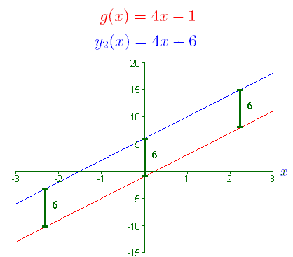
Figure 2- Changing Y-intercept (University of Arizona, 2018)

Implementation

HMI

The municipality was using RSView32 HMI that already had an ethernet link to the SLC PLC. A simple new screen was created with a connection to the setpoint of the PID loop. The operators could then fine-tune the setpoint with ease. Security was also added allowing only the operators with permission to adjust the setpoint.

Controls

The Cl₂ valve was wired to a spare I/O and tied to the CO of the PID – the flow and Cl₂ residual was already wired to the PLC. Logic for the feed-forward control, slope implementation, turbidity and PID were implemented and then tested. The PID was given the starting values that were calculated with the Cohen-Coon formula, with minor adjustments made at runtime. The flow rate and Cl₂ residual were added to the OSI PI historian for verification of performance.

Conclusion

A couple of months of historical data showed that the new system was operating much closer to the residual setpoint. The lead operators let me know that the Cl₂ levels were more constant through-out the water system and as a result the Cl₂ gas bill was reduced. This also brought about a higher level of safety for the end consumer; too little residual and the bugs don’t die, too much and there are health concerns. Adjustment of the setpoint was much easier than before and overall the project was a success.

References

Coughran, M. T. (2018, May 25). Retrieved from ControlGlobal: https://www.controlglobal.com/assets/13WPpdf/131022-coughran-controllers.pdf
University of Arizona. (2018, May 25). BioMath: Transformation of Graphs. Retrieved from http://www.biology.arizona.edu/biomath/tutorials/transformations/verticaltranslations.html